This is the first installment of a multi-part series of blogs that discusses feedback loop control design concepts, analytical methods and design tradeoffs. Although we will use power supply examples, the concepts (as Dean Venable oft reminds us) apply to all servo loops. We will do this with a minimum of math, and focus on developing an intuitive understanding of system behavior. For a deeper dive into this topic, please read Wayne Tuttle’s paper "Relating Converter Transient Response Characteristics to Feedback Loop Control Design". In this installment, we compare and contrast graphical analytical methods.

“Reading the Tea Leaves”

Graphical analytical tools have been a mainstay in engineering, and in this blog, we will examine two common tools, the transient response and the Bode plot. Both tools have been used to provide an understanding of system behavior, but the underlying system attributes are not fully revealed by either one. We will examine the system attributes, expressed as poles and zeroes, and how they manifest themselves in transient response Bode plot analyses.

The transient response analysis is typically an observation of system response to change. The change can be at the power supply’s input voltage or load (rarely does the power supply’s reference voltage change, but for servo loops, the set point does change and that results in a transient response). The transient system response is observed as a function of time, and results in a graphic representation as shown in Figure 1.

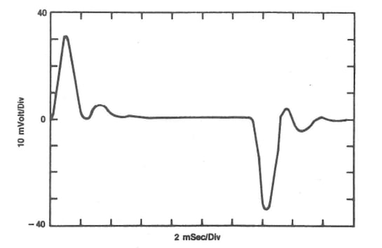Figure 1. Typical Transient Response.

If we want to observe system behavior in a different manner, we can look at the frequency domain. The Bode plot also describes system response, but does so as a function of frequency. Two system characteristics, gain and phase, are typically shown on the same plot, as shown in Figure 2.

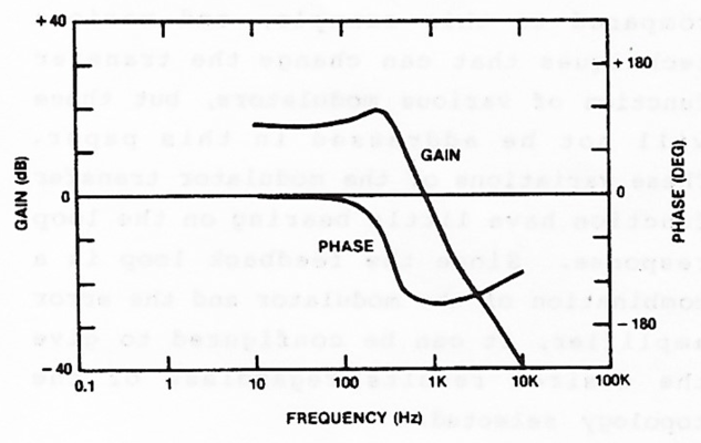Figure 2. Typical Bode plot showing gain (dB) and phase (degrees).

The system behavior is the Transfer Function, which can be expressed mathematically, but we are focusing on graphical analysis. The Transfer Function is a collection of poles and zeroes, and understanding their manifestation is key to understanding system behavior. It is difficult, nigh impossible, to account for environmental variables (e.g. temperature change resulting in a pole or zero moving) or parasitics (e.g. capacitor ESR, a parasitic zero) in a mathematical representation of the transfer function. However, graphical analysis gives us insight that accounts for all transfer function variables (poles and zeroes), and whether their effect is intentional or unintentional.

The transient response (a time domain representation) shows us how the system responds and the Bode plot (a frequency domain representation) shows us the why. With respect to system stability, the gain and phase Bode plot is the best (some would say only) graphical analytic tool. However, the gain and phase Bode plot alone does not tell us the whole story for system behavior. It will suggest (based on phase margin), that there might be overshoot or ringing due to a transient, but not how much or how severe. The transient response graphical analysis will tell us how much overshoot or ringing there is, but only suggest if a system is stable.

In the next installment, we will examine the plant and compensator (modulator and feedback), and how they manifest themselves using the transient response and Bode plot graphical tools.

If you cannot wait for the next installment, please read Wayne Tuttle’s paper "Relating Converter Transient Response Characteristics to Feedback Loop Control Design."