This is the second installment of a multi-part series of blogs that discusses feedback loop control design concepts, analytical methods and tradeoffs. Although we will use power supply examples, the concepts (as Dean Venable oft reminds us) apply to all servo loops. We will do this with a minimum of math, and focus on developing an intuitive understanding of system behavior. In this installment, we examine the transfer function a system to be controlled (the “plant”), and how it manifests itself in the frequency domain. It is imperative to fully understand the plant’s behavior in order to implement an effective feedback loop.
“The Transfer Function of the Plant”
In the first installment, we discussed two graphical analytical methods, the transient response and the frequency response, and how the two methods show us how and why the system responds the way it does. In this installment, we will dive deeper into the plant to be compensated, and the plant’s transfer function (poles and zeroes). We will see how the poles and zeroes manifest themselves on a Bode plot, both expected and unexpected.
For this discussion, we will use a simple buck regulator (for more information on power supply topologies, read Stability Analysis of Feedback Loops-Part 2) without any feedback. The regulator schematic is shown in Figure 1.
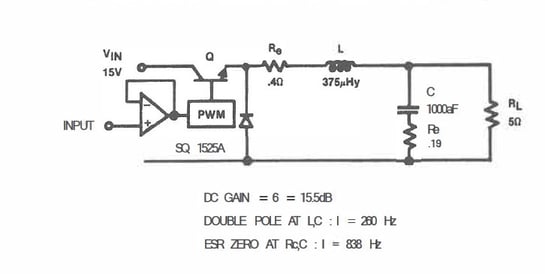
Figure 1. Buck regulator example (voltage control mode, continuous inductor current).
In power supply jargon, this is the modulator (more generically, the plant). The input controls the duty cycle (pulse width), where 0V in results in a zero percent duty cycle (0V out at RL) and 2.5V results in 100% duty cycle (15V out at RL). Since gain is defined as VOUT divided by VIN, we see that out plant has gain (2.5V/15V=6) at DC.
What happens if the 15V starts changing? Without compensation, we will see those changes at the output (RL). If we apply an AC voltage to the input of the switching transistor (Q), we will see an AC voltage at RL, but it will be affected by the reactive components L and C. The resulting Bode plot of the plant (modulator) is shown in Figure 2.
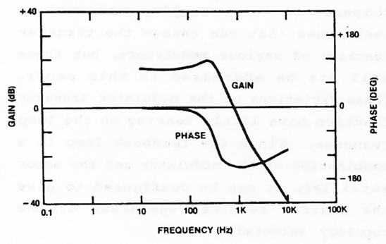
Figure 2. Modulator Gain and Phase Bode plot
So now we can observe the nature of the plant (modulator) as a function of frequency. Given that the gain and phase change over frequency, we can infer that the plant has poles and zeroes. When we analyze the Bode plot, it is possible to ascribe its gain and phase performance to plant elements (modulator components) as shown in Figure 3.
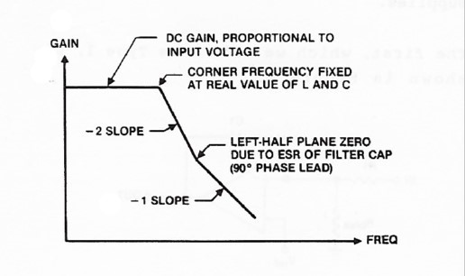
Figure 3. Modulator Bode Plot with Component Contributions
We can now see the two poles due to the inductor and capacitor on the output of the regulator affecting gain as a function of frequency. Additionally, we can see the zero that results from the ESR of the same capacitor that contributes a pole. We expected to see the two poles in the modulator Bode plot; they are intentional. However, the zero is a parasitic contribution and unintended.
So, in our example, we have characterized the plant (modulator) to be compensated and discovered (through frequency response analysis) that the transfer function contained a bit of a surprise. Not to worry, though, because with proper compensation we can tame the plant and get it to behave the way we want. Transfer function measurements of active and passive circuits/systems are easily accomplished with a Frequency Response Analyzer. If we did not have such insight to the plant’s behavior, taming it would inevitably be a heuristic process.
In the next installment, we will pick up with our example and determine the compensation needed and the effects that it can have on transient performance.
If you cannot wait for the next installment, please read Wayne Tuttle’s paper "Relating Converter Transient Response Characteristics to Feedback Loop Control Design."