Nyquist's 1933 paper on regeneration stated that a feedback control system could, at some frequencies, have 360 degrees of phase shift and more than unity gain without instability. At first glance it appears that this cannot be true. At these frequencies, the signal would progress around the loop and come back in phase and larger in magnitude - thus regenerating, or so it would seem. Systems with these characteristics can indeed be stable and are found with regularity in industry. This paper will explain clearly and simply what really happens in both conditionally and unconditionally stable feedback control systems, and how a loop attenuates with any gain other than unity.

INTRODUCTION
In 1933, Nyquist described criterion for stability in feedback control systems. He referred to them being either conditionally or unconditionally stable depending on the gain and phase shift characteristics. Many engineers feel uncomfortable with conditional stability and even doubt its existence. Nevertheless, it is actually common in power supply and servo control loops. It is important to understand how conditionally stable systems function so that they can be properly dealt with.

In some cases a conditionally stable system may be acceptable. A good fundamental understanding of the mechanisms involved with conditional stability is needed to make this decision. Before we get into this too far, let's review the basics and terminology that will be used in this paper.

WHAT ARE FEEDBACK CONTROLS?
A feedback control system is a device designed to hold some controlled variable constant. It does this by sensing the actual value of this variable, comparing it to a reference level, and correcting as necessary. This controlled variable may be torque, velocity, voltage, current, temperature, acceleration, or almost anything else that we might want to control. There is not much difference between the speed governor for a generator turbine at a hydroelectric power plant and a DC to DC converter. What we have is a DC servo loop. By modulating the reference with AC, DC servos can control AC signals.

The one thing that is common to all these systems is negative feedback. It should be clear that a system with negative feedback is inherently stable. A system with positive feedback will oscillate. If a system has negative feedback and, at some frequency, an extra 180 degrees of phase lag, it now appears to have positive feedback. If, at this frequency, there is a gain of 1 in the loop, the circuit will oscillate. The system will not oscillate if there is greater or less than unity gain in the circuit at the frequency where the total phase shift (counting the 180 degrees from the inversion) is 360 degrees. 

WHAT ARE NYQUIST DIAGRAMS AND BODE PLOTS?
Nyquist gave us a useful way to graphically depict the stability of a control loop. The NYQUIST
DIAGRAM is a polar plot giving phase and magnitude of voltages in a feedback loop. Figure 1 is a Nyquist diagram of an unconditionally stable system.  V1 represents the input voltage to the loop.

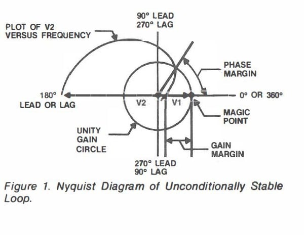
V2 represents the output voltage after going around the feedback loop. Notice that at DC the signal is amplified and inverted (180 degrees of phase shift). At higher frequencies, the amplitude of V2 decreases and the phase lag increases. The track that represents the head of the vector V2 is shown in this figure. Amplitude is proportional to the length of the vectors, and phase shift is proportional to the angles of the vectors. A unity gain circle is shown, which is the circle of all vectors that have the same amplitude as V1. When the amplitude of V2 is the same as V1, the difference between the actual phase shift and 360 degrees is the PHASE MARGIN. When V2 is in phase with V1, the ratio of the amplitude of V2 to V1 is the GAIN MARGIN.

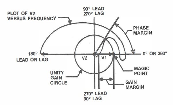
Figure 2. Nyquist Diagram of Conditionally Stable Loop

Figure 2 is a Nyquist diagram of a conditionally stable system. This figure is similar to figure 1 except that the phase of V2 shifts completely through 360 degrees and then back to less than 360 degrees before it crosses the unity gain circle. The magic point in this figure is the point where the unity gain circle crosses 360 degrees. Nyquist put this magic point at what he called" -1", and stated that stability was based on 180 degrees of phase shift. He chose to neglect the 180 degrees caused by the inversion (negative feedback). He only discussed the phase shifts that were associated with time lags. Nyquist pointed out that if the track of the V2 vector goes around this magic point in a counter-clockwise direction, the circuit is stable. Conditional stability is defined as the feedback loop having more than one point where the phase shift is 360 degrees.

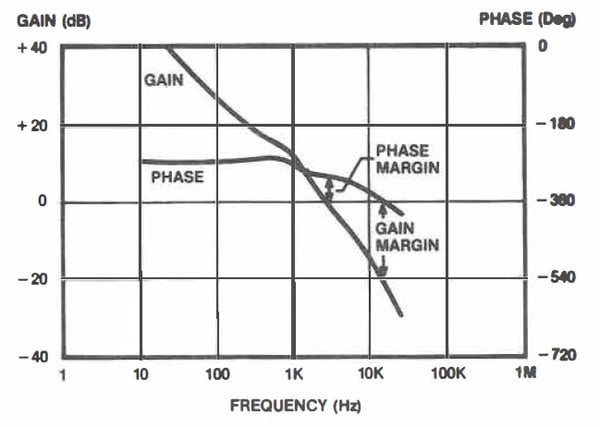Figure 3. Bode Plot of Unconditionally Stable Loop

Figure 3 is a typical BODE PLOT of an unconditionally stable system. A Bode plot is a plot of., log gain and linear phase versus log frequency. A useful way to configure Bode plots is to have O dB (unity gain) and 360 degrees (also O degrees) coincide. This allows phase margin to be read directly at gain crossover and gain margin to read at phase crossover. There are some interesting features of Bode plots concerning the slope of the gain curve as it relates to the phase shift. If the gain is flat with frequency, it is said to have a O slope. If the gain falls at 20 dB per decade (6 dB per octave) it is said to have a -1 slope. Gain falling at 40 dB per decade (12 dB per octave) has a -2 slope and so on. There is a definite phase shift associated with each slope. A O slope typically has O phase shift. A -1 slope has 90 degrees of phase lag. A
-2 slope has 180 degrees more phase lag than a 0 slope. Each minus slope change adds an additional 90 degrees of phase lag. Each plus slope change removes 90 degrees of phase lag. The actual amount of phase shift at any particular frequency is dependent on how near the comer frequency it is. Far away from corners the phase will settle in on the proper shift for its gain slope. Circuits that invert, such as an inverting amplifier have 180 degrees from the inversion and -90 degrees from its gain slope for a total of -270 degrees of phase shift. It is beneficial to configure Bode plots to have a factor of 10 in frequency (one decade) be the same dimension as a factor of 10 in gain (20 dB). In this way, slopes can be read and compared easily and a -1 slope is a 45 degree angle on the plot.

WHAT CONSTITUTES A LOOP?
There are at least two pieces that make up a loop. The MODULATOR or PLANT, and the ERROR AMPLIFIER. For clarity, we will define the modulator as being the power processing circuitry. Another way of describing the modulator is say it is everything except the error amplifier::, This allows us to design the error amplifier while using one set of data from the modulator. In this paper the sample control system is a switch-mode power supply. It could have also been a mechanical servo system. The same techniques and definitions apply. Figure 4 is a Bode plot of the modulator of the power supply. This plot is from the compensation pin of the pulse width modulation chip (SG1525A).

Figure 4. Bode Plot of Modulator Only

The plot has fixed gain (15.5 dB) at DC. At 260 Hz the gain starts to fall off due to the low pass filter used to smooth the chopped output of the switching transistor into pure DC. This gain is falling at a -2 slope and the phase starts shifting toward -180 degrees. It does not shift all the way to -180 due to the equivalent series resistance of the output filter capacitor. This causes the filter to become a L-R filter at high frequency instead of an L-C filter. The gain now falls at a -1 slope and the phase begins to shift back to -90 degrees. At higher frequencies time delays will cause the phase shift to become more negative. The amplifier will be designed to have the appropriate amount of gain and phase shift with frequency to allow the overall loop to have desired stability margins and performance. Figure 5 depicts an error amplifier that has phase boost. This boost in phase is caused by the change in the gain slope. This type of amplifier configuration can have up to 90 degrees of phase boost. When this error amplifier

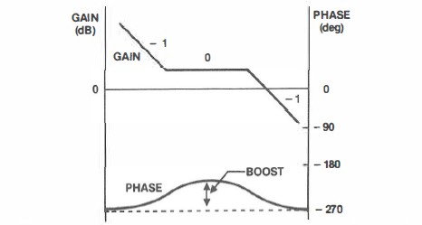Figure 5. Transfer Function of Error Amplifier with Phase Boost

is connected to a modulator, a composite, or overall loop plot can be created by simply adding the phase shifts and multiplying the gains. Since the gain is expressed in decibels, adding is equivalent to multiplication. The product is the loop gain of a closed loop system.

Figure 6 is a Bode plot of a conditionally stable system. The phase passed through 360 degrees three times, twice while there was gain in the loop and once while there was loss in the loop. The phase margin is still measured at the point where the loop gain is unity. Few design engineers intentionally design conditionally stable loops. They are usually the result of design errors or misunderstanding of circuit behavior. It is easy to see how they can occur in practice. The design engineer chooses a crossover frequency above the L-C corner frequency to make the loop to actively damp potential ringing of the output filter. If the slopes of the modulator and amplifier add to -3, then the phase shift will tend toward -450 degrees. The phase will not usually get all the way to -450 as the zeros in the amplifier will usually reduce the overall loop gain slope to -1 at crossover, which should yield a stable system. If the gain slope is -3 for enough of a range of frequency, the phase shift will get to 360 degrees as in Figure 6. An interesting thing about conditionally stable systems is that they have good transient response behavior. This is due to the steeper gain slopes. With these steeper gain slopes, the total area of gain under the gain curve as well as the actual gain at specific low frequencies is increased. When trial and error methods of compensation are used, it is easy to create a system that is conditionally stable. Let us look carefully at what seems to happen in conditionally stable systems and what really happens in all feedback control systems.

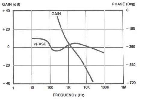Figure 6. Bode Plot of Conditionally Stable Loop

WHAT SEEMS TO HAPPEN IN CONDITIONALLY STABLE LOOPS?
Let us discuss what appears to happen in a typical conditionally stable system. In Figure 6 the phase shift is 360 degrees at several frequencies. At 800hz the gain is 10 dB with 360 degrees of phase shift. If a signal at 800hz passes through this circuit it will be phase shifted 360 degrees and amplified. It would seem that this would cause oscillations to occur since the signal will come back around the loop in phase with itself and larger in amplitude. Then the echo would pass around the loop, be further amplified and once again come back in phase. This explanation would then lead to the incorrect conclusion that the system will oscillate. While this seems to make sense, it would mean that conditional stability is an impossibility. Yet we can easily see that the system is stable and has excellent transient response characteristics as shown in Figure 7. This should indicate that there is something wrong with the logic that led to this conclusion. We are improperly predicting closed loop response from open loop transfer functions.

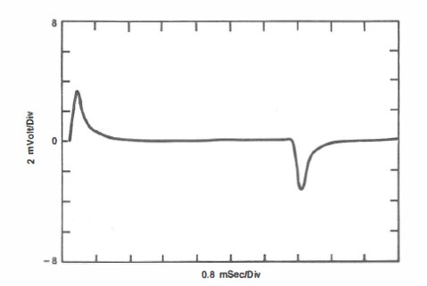Figure 7. Transient Response of Conditionally Stable System

WHAT REALLY HAPPENS IN LOOPS
Let's look at how the system actually regulates. At the heart of the system is the error amplifier. In this example it is an inverting amplifier. If there is an inversion elsewhere in the circuitry the amplifier will not be an inverting amplifier. Good practice usually requires the amplifier to be inverting as it provides the most design flexibility for the design engineer. This is because the gain of a non-inverting amplifier can only fall to unity. This error amplifier is what allows the system to regulate. It compares the output to a known reference and amplifies the difference, and drives the input of the modulator, causing correction of the error. As was discussed earlier, there is phase shift associated with this inversion as well as the gain slope. These phase shifts are different indeed. The inversion is just that: an immediate inversion of the input signal polarity. The phase shift of the gain slope is a phase lag. It posses(a "time shift" or delay that causes the phase lag. There is no delay associated with the inversion. Now let's bring gain into the picture. If there is gain in the loop, this indicates that the loop has the ability to correct for the error. This is because the error signal from the output of the error amplifier will pass through the loop, be multiplied by the modulator gain, and have sufficient magnitude to eliminate the error. If there is unity gain, or gain less than unity, the system will not be able to swing its output enough to correct for errors caused by transients or other perturbations. Above the crossover frequency, it will attenuate signals passively because the gain is less than unity and the error is reduced on each successive pass around the loop. The active rejection of the transient occurs only when there is gain in the loop. This means that there are three different ways that AC signals are handled by the feedback loop. When there is loop gain greater than unity, the signals are actively rejected. When the gain in the loop is less than unity the signals are passively attenuated. When the gain is unity the signals pass seemingly unimpeded around the loop. For this reason systems with 360 degrees of phase shift will oscillate only with unity gain. The signal will be of the same amplitude and in phase with itself and there will be no attenuation. If there is phase margin (total loop phase shift less than 360 degrees) there will be attenuation of the signals due to the misalignment of the echo signal caused by the phase margin. This misalignment causes the amplitude to be lower, in the direction of change, at any given point in time although the actual AC value is the same.

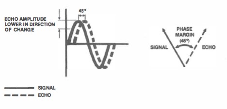
Figure 8. Attenuation due to Phase Shift at Unity Gain

This is shown graphically in Figure 8. The greater the phase margin, the greater the rejection of the potential oscillations at the unity gain frequency. To see what happens with 360 degrees of phase shift and gain in the loop, we first have to look at the output of the error amplifier. Figure 9 shows the input and output of the error amplifier when a square wave transient is applied. Because of the lack of time delay associated with the inversion, we can see that the output always ramps immediately in the correct direction. The gain and phase shift will have an effect on the slope of the ramp, but the direction that the output is ramping is always right. If the gain in the loop is greater than unity, then the system will have the ability to reject errors because the gain of the error amplifier causes sufficient swing of the input of the modulator to cause the output of the system to correct for the transient. The phase shifts will affect the slope of the output swing, but the direction of this swing will be in the direction that causes rejection rather than regeneration. 

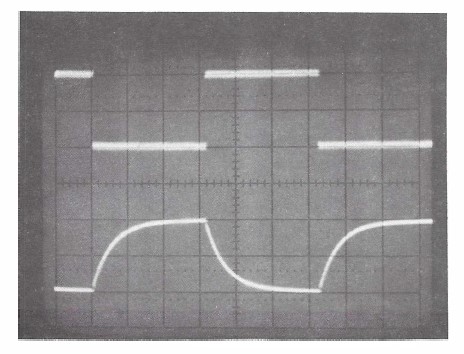Figure 9. Input and Output Waveforms of Error Amplifier

WHAT IS SO BAD ABOUT CONDITIONALLY STABLE SYSTEMS?

We have shown that conditionally stable systems are indeed stable and will reject transients and other perturbations quite well. Since the gain slope is steeper, and the gain at any given frequency below loop gain crossover is higher, the transient response for a conditionally stable system is faster than an unconditionally stable system of equal phase margin and crossover frequency. This makes the conditionally stable system seem to be the better choice. This would be true if the gain never changes in the system. An unconditionally stable system will be stable unless the gain is increased by the amount of the gain margin. In actual practice it is unusual for the gain to increase in the operation. On the other hand it is common for the gain to be decreased at certain times of operation. If any part or section of the system becomes saturated the gain will fall. If the output is slew rate limited, the gain will fall during the response to certain transients. If the system in question is unconditionally stable, the loss of gain will not cause instability and often will increase the phase margin due to the resulting lower crossover frequency during the response itself. If this system is conditionally stable these same gain reducing situations can cause instability. Conditionally stable systems are stable only when the loop gain is within a certain range. This stable range can be violated not only during large signal transient response, but during power up, low line, and other temporary conditions. If a conditionally stable system is subjected to sufficient temporary decrease in gain, the system will oscillate. This oscillation may cause saturation within the system, preventing the gain from increasing to the point where the system would achieve stability. These oscillations may result in damage to the system. 

HOW TO AVOID CONDITIONALLY STABLE DESIGNS
The only way to be certain that a system is unconditionally stable under all operating conditions is by measurement of the loop gain and phase shift under actual operating conditions or accurate modelling. The trouble with modelling comes in creating an accurate model that truly reflects the system including parasitic elements. These are often overlooked in the original model. An example of this type of element is a time delay which appears as a phase shift that increases with frequency. Through the interaction of test data and model data, accurate modelling can be done that will assist in the determination of stability. Simply connecting a step load to the system under test and optimizing the transient response is not enough. We often find systems that have excellent transient response and yet have poor stability margins and are potential field failures.

SUMMARY AND CONCLUSIONS
Conditionally stable systems are indeed stable and can possess good transient response. They are easily created when step response is the criteria used for loop optimization. They are stable under certain conditions, but if these conditions are violated, as in large signal response, there is an opportunity for instability. They are capable of response with loop gain and 360 degrees of phase shift because of the instantaneous inversion in the loop that causes the response to occur in the right direction for rejection. The phase shift in the loop, when there is gain greater that unity, will affect the slope of the ramp involved with the corrective action. Conditionally stable systems should be used only when the gain cannot be depressed in actual operation. The best way to assure stability in a control system is to measure loop gain and phase shift in actual operating conditions.

BIOGRAPHY
Mr. Tuttle is a member of the technical staff at Venable Industries, Inc., the leading manufacturer of complete frequency response analysis systems. He is a well-known consultant and lecturer and has authored several papers on the subject of feedback control optimization. 

REFERENCES 

1)Nyquist, H., "Regeneration Theory", Bell Systems Tech. J., vol. II, pp. 126-147, 1932.
2) Venable, H. Dean, "Practical Techniques for Analyzing, Measuring and Stabilizing Feedback Control Loops in Switching Regulators and Converters", Proceedings of the Seventh National Power Conversion Conference, POWERCON 7, pp. 12-1 to 12-17, March, 1980.
3) Venable, H. Dean, "Stability Analysis Made Simple", Torrance, CA, Venable Industries, 1982.
4) Venable, H. Dean, "The K Factor: A New Mathemati­cal Tool-For Stability Analysis and Synthesis", Proceedings of the Tenth International Power Conversion Conference, POWERCON 10, pp. H1-1 to H1-12, March 1983.
5) Tuttle, Wayne H., "Relating Converter Transient Response To Feedback Loop Control Design", Proceedings of the Eleventh International Power Conversion Conference, POWERCON 11, pp. E1-1 to E1-14, April 1984.