Tuttle’s Topics

This is the final installment of a multi-part series of blogs that discusses feedback loop control design concepts, analytical methods and tradeoffs. Although we will use power supply examples, the concepts (as Dean Venable oft reminds us) apply to all servo loops. We have done this with a minimum of math, and focused on developing an intuitive understanding of system behavior. In the final installment, we summarize the concepts used to close the loop and achieve desired design behavior.

“Wrapping Up”

In previous installments, we have discussed graphical analytical methods, how and why the system responds the way it does, and how feedback affects the closed loop performance. In this installment, we will review all the pieces of the puzzle and how they fit together. We started with graphical analysis and how the any system can be observed in both the time domain (transient response) and frequency domain (Bode plot). Examples of both are shown below (Figure 1.) 

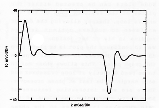
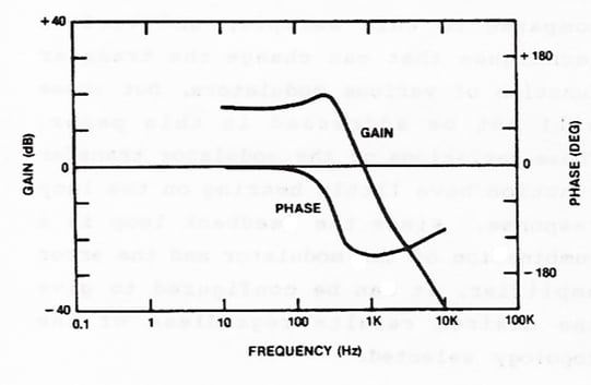Figure 1. System Transient Response (top) and Bode plot (bottom)

Both graphs represent the same system, but the Bode plot can reveal the why. All systems are a collection of poles and zeros (mathematical concepts) that are a result of real-world characteristics. A closed loop system with negative feedback can be divided into the plant (modulator in power supply terms) and compensation (feedback). Understanding the plant’s behavior is the first step in implementing the proper feedback. In our power supply example, the poles and zeros resulted from the arrangement (topology) of the electronic components and their parasitics. We do have choices regarding topologies and components, but those choices are somewhat limited by the overall function of the plant (the plant has to implement our desired function).

The interesting aspect (the fun part) of compensation is implementing additional poles and zeroes so that the system (plant + compensation) has the desired behavior. How many poles and zeroes and where to put them is easily determined by the K Factor analysis. The analysis allows us manipulate the closed loop performance (often referred to as the “loop gain”) to achieve the desired behavior, expressed in terms of gain and phase (which are revealed in a Bode plot). In the time domain we can go from this (Figure 2.),

To this (Figure 3.).

For a deeper dive into understanding the concepts of frequency domain analysis and compensation, please see Wayne Tuttle’s paper, "Relating Converter Transient Response Characteristics to Feedback Loop Control Design."

There are many hefty textbooks written on the subject of control theory and feedback, but in this series of blogs, we have tried to boil it down to easy to grasp pieces. The transient response of a system is a reflection of its frequency response and both are important analytical tools. Viewing any system’s frequency response allows us to understand the system’s intrinsic nature and manipulate it. Venable Instruments has embraced this concept and developed the tools for engineers to understand and manipulate any servo loop. Venable’s Frequency Response Analyzers and Stability Analysis Software are the industry benchmark and are essential to any engineer’s toolbox.

Tuttle's Topics #4 Closing the Loop - Feedback Circuits

Tuttle's Topics #3 Closed Loop Performance

Tuttle's Topics #2 - Measure and Know Your Plant

Tuttle's Topics #1